Clinical Risk Prediction with Logistic Regression: Best Practices, Validation Techniques, and Applications in Medical Research

Introduction

Clinical medicine relies on data derived from a variety of sources, including patient interviews, physical assessments, laboratory tests, and imaging studies.¹ These data are compiled in numerous formats and can be broadly categorized according to variable type—for instance, continuous measures (e.g., serum cholesterol levels), categorical classifications (e.g., presence or absence of a disease), nominal groupings (e.g., blood type), or ordinal scales (e.g., disease severity scores).² The choice of an appropriate analytical method depends heavily on these variable types: certain statistical techniques are more suitable for continuous variables, while others are better suited to categorical or ordinal data.³ When data collection or storage is inconsistent—for example, misclassifying a continuous variable as categorical—analyses can become flawed, resulting in biased or incorrect conclusions, and undermining the reliability of research findings.⁴

Clinical research studies typically employ designs such as prospective and retrospective cohorts, as well as case-control studies. Each of these designs calls for a tailored approach to analysis.⁵ Prospective cohort studies collect data going forward in time to observe outcomes, often enabling stronger inference regarding temporal relationships. Retrospective cohorts draw on existing records to examine outcomes that have already occurred, requiring careful attention to data completeness and potential biases in record-keeping. Case-control studies, by contrast, start with the identification of cases (individuals with a particular outcome) and controls (those without the outcome), and then look back in time to identify explanatory variables.⁵ Because each study design has its own strengths, limitations, and typical analytical strategies, recognizing how data were gathered is essential for selecting valid and meaningful statistical methods.

In many clinical research scenarios, the choice of method becomes more straightforward when all variables share the same type (e.g., multiple continuous variables). However, researchers commonly face situations where the independent variable (x) is continuous—such as blood pressure or a biomarker concentration—and the dependent variable (y) is categorical—such as “disease present vs. disease absent.” Logistic regression is frequently used to address this type of question; it provides a way to estimate the probability of a particular outcome (e.g., the presence of disease) in relation to one or more predictors, making it especially valuable in diagnostic, prognostic, or risk-factor analyses.⁶

A concrete example of logistic regression’s utility can be seen in studies that predict whether patients with chest pain are likely to have an acute coronary syndrome.⁷ Using factors like troponin levels, blood pressure, and electrocardiogram findings—each of which may be measured on different scales—a logistic regression model can estimate the probability that a patient truly has a significant cardiac event.⁸ This kind of approach helps clinicians triage patients quickly and allocate resources more efficiently. Without a sound logistic regression framework, such data might be analyzed incorrectly (for instance, by treating these variables as if they were all continuous and had a linear relationship to the probability of disease), leading to suboptimal or misguided clinical decisions.⁹

Beyond these foundational considerations, it is important to recognize that logistic regression comes with several key assumptions that must be met for valid inference. Chief among these is the assumption that the log-odds of the outcome are linearly related to the predictor variables.¹⁰ Violations of this assumption can lead to model misspecification and misinterpretation of results. Logistic regression also outputs odds ratios, which reflect the change in the odds of an outcome for a one-unit change in a predictor variable.^11,12 While odds ratios are incredibly useful in clinical settings, equating them directly to risk ratios or interpreting them without regard to baseline probabilities can lead to misleading conclusions about a disease’s absolute risk.^11,12

A further consideration is that misuse of logistic regression—such as neglecting confounding variables, failing to check for multicollinearity, or inadequately handling missing data—can undermine the validity of research findings and contribute to flawed clinical decision-making.¹³ Conversely, when properly applied and validated, logistic regression plays a critical role in informing treatment strategies, screening protocols, and the allocation of healthcare resources. Its relatively straightforward interpretability, as well as the ability to incorporate p-values and confidence intervals, sets logistic regression apart from more complex machine learning approaches, making it a staple in evidence-based medicine despite the emergence of alternative modeling techniques.¹⁴

This narrative review focuses on the proper uses, applications, and validation of logistic regression in clinical medicine. We will explain how and when logistic regression is most appropriate, outline the key variable types involved, address common misconceptions about the method, and differentiate the nuances of univariate versus multivariate modeling. Finally, we will discuss strategies for developing, validating, and testing logistic regression models to ensure they are both robust and generalizable across a range of clinical settings.

Methods

This study is a narrative review of 41 papers published between 1987 and 2025 focusing on the use of logistic regression in clinical research. We chose a narrative review approach to synthesize findings from a broad array of study designs and clinical contexts, rather than following the stricter protocols of a systematic review. We conducted an initial literature search using the databases PubMed, MEDLINE, and Scopus, combining the keywords “logistic regression,” “clinical medicine,” “medical research,” “diagnostic studies,” “prognostic models,” “retrospective,” “prospective,” and “odds ratio.” We included both primary research articles and review papers that discussed the applications, assumptions, and validation techniques associated with logistic regression in a clinical setting.

During the selection process, we screened titles and abstracts to identify studies that directly employed logistic regression for analyzing categorical outcomes (e.g., presence/absence of a disease) and addressed core assumptions (e.g., linearity in the log-odds). We also sought examples illustrating both best practices and common pitfalls—such as failing to account for confounding variables, misinterpreting odds ratios, or not verifying model fit. Articles focusing solely on non-clinical contexts (e.g., business applications) or on other statistical methods without substantial mention of logistic regression were excluded. Each author then independently reviewed the full text of the included articles, extracting information on study design, model-building strategies, validation processes, and interpretative guidelines. Findings were subsequently cross verified in collaborative discussions, ensuring consistency and completeness in our synthesis.

Because this is a narrative review, we did not perform a formal meta-analysis or statistical pooling of results. Instead, we integrated and summarized key themes that emerged across studies, noting both methodological rigor and frequent analytical challenges. The main areas of focus included: (1) the role of logistic regression in different study designs (prospective and retrospective cohorts, case-control studies), (2) best practices for data preparation and variable selection, (3) interpretation of logistic regression outputs (particularly odds ratios), (4) strategies for checking model assumptions (such as linearity in the log-odds and absence of perfect separation), and (5) methods of model validation (e.g., calibration, discrimination, cross-validation). We also compiled examples illustrating how authors dealt with real-world issues like missing data, collinearity, or small sample sizes. Through this process, we aimed to create a cohesive, clinically oriented review that is relevant to physicians, researchers, and other healthcare professionals interested in the robust application of logistic regression.

Discussion

Concepts of Logistic Regression and When to Use

Logistic regression aims to predict the probability of an event occurring based on a linear combination of predictor variables.⁹ Because of this, it requires the dependent (y) variable to be a binary outcome (i.e. 0 or 1, positive or negative for a disease). The independent (x) variable(s) may be continuous (e.g. BMI, hematocrit) or categorical (e.g. gender, ASA Class), however at least one of the independent variables must be continuous. If the goal of your analysis is to predict the probability of an event occurring or not, using continuous data as a predictor, logistic regression may be an appropriate model.⁹

Linear regression is easily understood for having the value you predict (y) be equal to a linear combination of the predictor (x) variables.¹⁵ This equation is shown below, where $\widehat{Y}$ represents the outcome, $X_{1 - k}$ represent the predictors, $\beta_{0}$ represents the Y-intercept, and $\beta_{1 - k}$ represent the coefficients.

$$\widehat{Y} = \beta_{0} + \beta_{1} X_{1} + \cdots + \beta_{k} X_{k}$$

Equation 1. Linear Regression.¹⁶

Since logistic regression aims to predict a probability, we will replace $\widehat{Y}$ with $\widehat{p}$ for probability. We then need to ensure that the value for $\widehat{p}$ remains between 0 and 1. We achieve this by applying the log-odds transformation to $\widehat{p}$, which results in the equation below.¹⁷ Again, $\widehat{p}$ represents the probability, $X_{1 - k}$ represent the predictors, $\beta_{0}$ represents the Y-intercept, and $\beta_{1 - k}$ represent the coefficients.

$$ln(\frac{\widehat{p}}{1 - \widehat{p}}) = \beta_{0} + \beta_{1} X_{1} + \cdots + \beta_{k} X_{k}$$

Rearranging, we can solve for $\widehat{p}$, which equals:

$$\widehat{p} = \ \frac{1}{1 + e^{- z}}\ ,\ \ where\ z = \ \beta_{0} + \beta_{1} X_{1} + \cdots + \beta_{k} X_{k}.$$

Equation 2. Logistic Regression.¹²

This transformation ensures that $\widehat{p}$ remains between 0 and 1 and gives us a sigmoid-shaped (“S”- shaped) curve representing the probability of an event occurring given a particular level of the predictor value. An example using high-sensitivity troponin to predict the likelihood of acute coronary syndrome (ACS) via logistic regression is shown in Figure 1.

Figure 1.Example of a univariate logistic regression model using high sensitivity troponin to predict the likelihood of acute coronary syndrome. *Note that this is fictional data and not intended to represent the true relationship between ACS and troponins. Graph is author’s own work.

Interpretation of Logistic Regression Output

When you successfully construct a logistic regression model, a table of output will typically be provided along with the equation and graph. This table of output contains valuable information about the accuracy, strength of association, statistical, and clinical significance of the model and as such, it is essential for the clinical researcher to understand the interpretation of these values¹⁸ (Table 1).

For example, let’s interpret the output of the prior regression using high-sensitivity troponin to predict ACS. Below is the output:

Model Fit Metrics:

• Pseudo R² = 0.28

• AIC = 190.2

Which has the following interpretation:

• A negative intercept (–3.50) implies that at near-zero troponin, the baseline probability of ACS is low.

• The coefficient of 1.20 (log-odds scale) translates to an odds ratio of ~3.32, meaning each unit rise in troponin multiplies the odds of having ACS by over three.

• The p-value < 0.001 in the troponin row and 95% CI well above 1 confirm that high-sensitivity troponin is a strong, statistically significant predictor of ACS.

• The pseudo-R² of 0.28 suggests that troponin alone explains why 28% of individuals in the dataset end up with or without ACS. This is generally considered a ‘good’ value in clinical studies.¹⁹

• An AIC of 190.2, by itself, doesn’t say “good” or “bad” in absolute terms; it mainly becomes meaningful when compared with the AIC of another logistic regression model predicting the same outcome.

Assumptions and Preconditions for Using Logistic Regression

As with most statistical models, logistic regression relies on a core set of assumptions and preconditions that the data must adhere to before the model can be reliably applied. Below, we examine each of the preconditions with an example from the prior ACS model.

1. Binary Outcome¹⁸

Assumption: The outcome variable (ACS) must be coded as 0 = no ACS or 1 = ACS (or similarly binary).

• Why it matters: Logistic regression models the probability of a binary event.

• How to check:

  • Confirm your data file has a clear 0/1 (or “no/yes”) coding for ACS.

  • If there are multiple categories (e.g., ACS subtypes), you may need different coding or a different analysis (multinomial logistic regression).

Example:

• Ensure the dataset has acs = 0 for non-ACS patients and acs = 1 for ACS patients.

2. Independence of Observations¹⁰

Assumption: Each data point (e.g., each patient) should be independent of the others.

• Why it matters: Standard logistic regression methods assume that no repeated measures or clusters of correlated data are present.

• How to check:

  • Confirm that each row in your dataset is from a distinct patient.

  • If repeated measurements or clusters exist (e.g., multiple admissions of the same patient), consider mixed-effects or other specialized models.

Example:

• Verify that each troponin measurement in your dataset comes from a different patient, so there is no repeated-measures structure (e.g., patient returning multiple times).

3. No Perfect Separation²⁰

Assumption: There should be no single predictor (or combination of predictors) that perfectly separates the 0 and 1 outcome groups.

• Why it matters: If troponin alone always 100% predicts ACS vs. no ACS, the model parameters can become infinite (the log-odds blow up).

• How to check:

  • Plot troponin vs. ACS status (0 or 1).

  • Look for a clean cutoff where all ACS=1 patients have troponin above X and all ACS=0 patients have troponin below X with no overlap. If that exists, you likely have perfect separation.

Example:

• If in your dataset, everyone with troponin >10 is ACS=1 and everyone with troponin ≤10 is ACS=0, you have perfect separation. Typically, that’s rare, but it can happen in small samples.

4. Log-Odds Linearity¹⁰

Assumption: Each predictor (e.g., troponin) is assumed to have a linear relationship with the log-odds of the outcome.

• Why it matters: Logistic regression is essentially linear in the log-odds space. If the relationship is nonlinear, the model may misfit.

• How to check:

  1. Transform troponin into categories (e.g., bins of troponin) and check if the log-odds of ACS change in roughly a straight-line fashion.

  2. Use polynomial or spline terms in the model to see if they significantly improve model fit.

  3. Partial residual plots to visualize if the log-odds appear linear.

Example:

1. Create bins for troponin (for example, 0–1, 1–3, 3–5, etc.).

2. Calculate ACS rates in each bin (i.e., the proportion of patients who have ACS in that bin).

3. Convert each proportion (ACS rate) to log-odds:

$$log-odds = \ ln(\frac{\widehat{p}}{1 - \widehat{p}})$$

4. Plot the log-odds of ACS against the midpoint of each troponin bin.

5. If these points roughly form a straight line, it suggests the log-odds relationship is linear—meaning the logistic regression model is a good fit for troponin.

5. No Strong Multicollinearity (for multiple predictors)¹⁰

Assumption: When using more than one predictor (e.g., troponin + blood pressure + age), those predictors shouldn’t be highly correlated with each other.

• Why it matters: Multicollinearity inflates standard errors, making the model coefficients unstable.

• How to check:

  • A simple linear regression can reveal whether two or more predictors are very strongly correlated (e.g., r > 0.8).

Example:

• If you’re modeling ACS with troponin, BNP, and creatinine, you’d check the correlation between troponin and BNP to ensure troponin isn’t extremely highly correlated with BNP (another cardiac biomarker). If they are, it may cause unstable estimates.

6. Adequate Sample Size²¹

Assumption: You need enough data (particularly enough events = ACS=1 cases) to reliably estimate coefficients.

• Why it matters: Too few cases with ACS leads to an overfitted model or inflated standard errors.

• How to check:

  • Rule of thumb: ≥10 events per predictor. If you have 1 predictor (troponin) and only 15 ACS patients out of 300, that’s generally acceptable. But adding more predictors would require more ACS events.

Example:

• If your dataset has 300 patients, 50 of whom have ACS, that’s generally enough to handle upto 5 predictors in logistic regression. If you want to add 6+ predictors, you might be pushing the 10-events-per-predictor rule. There is, however, evidence in certain cases to allow for this.²¹

Multivariate Logistic Regression

Multivariate logistic regression is an extension of simple (univariate) logistic regression that models the probability of a binary outcome (such as disease vs. no disease) using multiple predictor variables. Instead of analyzing the effect of a single factor—like one biomarker—on the odds of having an outcome, multivariate logistic regression incorporates a set of predictors (e.g., age, blood pressure, biomarker levels, comorbidities) all at once.²² By doing so, it can control for confounding variables and tease apart the individual contribution of each predictor while holding others constant.²³ This is particularly valuable in clinical research, where patients often present with a combination of risk factors, and the relationship among those factors can be complex. Multivariate logistic regression helps researchers and clinicians identify which variables are the strongest drivers of a given outcome, improve risk stratification, and make better-informed decisions about patient diagnosis and management.²³

Multivariate logistic regression utilizes the same equations presented above (Equation 2), and requires coding binary predictor variables (e.g., smoker or non-smoker) as 1 or 0 (e.g. smoker = 1, non-smoker = 0). Similarly, ordinal predictor variables that are not continuous but have an order to them, such as ASA class, must be coded as 1-6 to fit into the model.²⁴

Generally, for a research manuscript, univariate models are constructed for each predictor variable and each potential confounding variable prior to constructing the multivariate model.²⁵ This allows the researcher to identify which variables are associated with the outcome of interest and include only those that are significantly associated with the outcome in the multivariate model. This helps to satisfy precondition #6, which states that you must have ~10x the number of positive events in your data as predictor variables.²¹

For example, in a study of 1,472 patients undergoing panniculectomy, investigators initially tested five predictors in univariate logistic regression for their association with postoperative wound infection: age, BMI, diabetes status, smoking status, and preoperative albumin. They found that lower albumin and higher BMI were significantly associated with an increased risk of wound infection (p < 0.01), while age, diabetes, and smoking did not reach significance. As a result, only albumin and BMI were carried forward into the multivariate logistic regression model, ensuring that the final analysis focused on the variables truly predictive of wound infection in this patient population.²⁶

Let’s interpret some sample output for the prior study, as shown below:

Interpretation

1. Albumin: A 1 g/dL decrease in preoperative albumin is associated with a log-odds coefficient of 1.61, corresponding to an odds ratio of 5.00. In other words, each 1 g/dL drop in albumin multiplies the odds of wound infection by five (95% CI: 2.70–9.20). The p < 0.001 indicates high statistical significance.

2. BMI: Each additional 1 kg/m² in BMI increases the log-odds of wound infection by 0.05, translating to an odds ratio of 1.05 (95% CI: 1.02–1.08). Although this effect is modest, it is still statistically significant (p = 0.003).

3. Intercept: Represents the baseline log-odds of wound infection when albumin and BMI are at zero (not clinically relevant as an absolute value, but important mathematically for the model).

Multivariate logistic regression allows the researcher to examine the effects of multiple different variables on a particular outcome and compare the relative association between them.²⁷ This allows the researcher to make an inference on how much a change in one variable matters. In the previous example, we can see that a decrease in 1g/dL of albumin increases the odds of wound infection by 5x, while an increase in one point of BMI only increases the odds of wound infection by 1.05x.

One way to think about that difference in effect sizes is to ask, “How many single-point increases in BMI would it take to have the same impact on infection odds as dropping albumin by 1 g/dL?” Mathematically, because each 1-point rise in BMI multiplies the odds by about 1.05, you need around 33 incremental increases for the product to reach 5 (i.e., (1.05)³³ ≈ 5). Practically, that means a huge change in BMI is needed to match the same fivefold jump in odds of infection that comes from a single 1 g/dL drop in albumin.

Why 33 BMI Points?

• The odds ratio (OR) for a 1 kg/m² increase in BMI is 1.05.

• To get the same total increase in odds (×5) as a one-unit drop in albumin, you solve the equation:

$${(1.05)}^{x} = 5\ \rightarrow x = \ \frac{\ln{(5)}}{\ln(1.05)}\ \approx 33.$$

• Interpreted literally, a 33-unit rise in BMI (e.g., from a BMI of 25 to 58) yields about the same multiplicative effect on the odds of infection as dropping 1 g/dL in albumin.

Real-World Caveats

• A 33-point BMI change is huge in clinical terms, so while the math is correct, it highlights that albumin has a substantially larger effect per “standard unit change” than BMI in this particular model.

• Always remember these are model-driven inferences; in practice, BMI changes of that magnitude are rarely instantaneous or linear, and albumin levels can shift for many reasons.

Still, the calculation helps illustrate how much bigger an effect (on the odds of infection) a 1 g/dL drop in albumin exerts relative to the effect of modest BMI increases.²⁶

Multivariate Examples

We have included some examples of how multivariate logistic regression is used in different ways in real-life scenarios, to emphasize accurate interpretation of the model in various scenarios.

Note: All examples, while based on real research, are hypothetical scenarios used to illustrate concepts of logistic regression in this manuscript and may not represent the true relationship between any variables mentioned.

Example 1: Using a Frailty Score to Predict Reintubation in Thoracic Surgery²⁸

Unplanned reintubation is a major pulmonary complication in thoracic surgery. You are interested in predictors of this outcome. Recently, the 5-item modified frailty index (MFI-5) has begun to be used in preoperative planning alongside the standard ASA classification at your hospital, and you want to evaluate the effect of MFI-5 in predicting reintubation in thoracic surgery. The MFI-5 separates frailty into five classes: 1, 2, 3, 4, and 5, much like the ASA classification.

A study was done evaluating MFI-5 in predicting reintubation and utilized a multivariate logistic regression model including MFI-5 and age, sex, smoking status, and preoperative steroid use, which were all found to be potential confounders in the univariate analysis. You are given the below output table.

Below is the interpretation:

• Older age was associated with a modest but significant risk increase, with an OR = 1.02 (p=0.001). This means the odds of reintubation increases by 2% each additional year of age.

• Moving from MFI 1 to 2 roughly tripled the odds (OR = 3.30, p<0.001).

• Each unit increase in the MFI from 0 to 1 to 2 to 3 resulted in different increases of odds. Moving from MFI 3 to 4 and 4 to 5, however, were not significantly associated with reintubation. This likely occurred due to small sample size of MFI 4’s and 5’s.²⁸

• Smoking raised the odds by 60% (OR = 1.60, p=0.01).

What if you wanted to know how much the odds of reintubation increase from MFI 0 to 2, a two-unit increase? Then you would need to multiply the odds ratios of MFI 0-1and MFI 1-2. This would equal 1.9 * 3.3 = 6.27. Thus, a person with MFI score of 2 has 6.27 higher odds of reintubation than a person with MFI score of 0, all else being equal.²⁸

Example 2: Determining if Convergence Insufficiency Predicts Hospital Admission for Post-Concussive Syndrome²⁹

You are interested in determining if convergence insufficiency (CI) predicts the likelihood of being admitted to the hospital for post-concussive syndrome (PCS) in mild traumatic brain injury (mTBI). The authors of the paper construct a multivariate logistic regression including a CI Symptom Survey (CISS) score and other emergency department (ED) variables. The output is shown below:

Below is the interpretation:

• Age: Each additional year of age increases the odds of hospital admission by about 4% (OR=1.039, p=0.015), making age a significant predictor.

• CISS Score: A higher convergence insufficiency symptom score strongly increases the odds of admission (OR=1.57, p=0.021), suggesting CI is a meaningful factor in post-concussive syndrome.

• Abnormal CT, Sex, and GCS: None reached statistical significance (p-values > 0.05), indicating they did not robustly predict admission in this sample.

In logistic regression, each “Estimate” reflects how much the log-odds of the outcome (in this case, being admitted) change with a 1-unit shift in the predictor. For sex, the estimate is –0.6406, which means:

• Being Female (Female = 1, Male = 0) lowers the log-odds of being admitted by 0.6406.

• In odds-ratio terms, that translates to an OR of ~0.53 ($e^{- 0.6406} \approx 0.53$), indicating that being female nearly halves the odds of being admitted for PCS.²⁹

Training, Validation, and Testing Data Sets

When building a logistic regression model (or any predictive model) it is important to divide your data into three parts: training, validation, and testing sets. This practice helps ensure that the final model is both accurate and relevant when caring for future patients.³⁰

1. Training Set

   • Purpose: This is the portion of data used to actually build the model. In a logistic regression, the computer “learns” what combination of clinical measurements (predictor variables) best predict the outcome of interest (e.g., complication vs. no complication).

   • How It Works: The model calculates and adjusts coefficients so that it can accurately predict the outcome for patients in the training set. If, for example, “age” and “lab value X” are important predictors, the training set helps the model “figure that out.”

2. Validation Set

   • Purpose: This subset helps you decide how complex the model should be and which predictors you truly need.

   • How It Works: After creating a preliminary model from the training set, you check how well it performs on the validation set. If the model works well on training data but does poorly on the validation data, it might be overfitting (memorizing details of the training set rather than learning the general pattern). You can then remove or adjust certain predictors based on these validation results.³¹

   • Example: You measure the accuracy of your model on the training data as 95%, but the accuracy on your validation set is only 69%. You notice that while BMI, diabetes, and hypertension all have p < 0.01 and an odds ratio well above 1.0, tobacco use only has p = 0.049 and an odds ratio of 1.02. You may choose to omit tobacco use in the model due to its borderline statistical significance and retrain your model on the training data without tobacco use. This process of training and validation is then iterated until the performance on the validation data is deemed acceptable (i.e. close to the training data).³²

3. Testing Set

   • Purpose: Once you have settled on your final model, you use the test set for a one-time check of how well that model performs on “new” patients.

   • How It Works: Because the test set was never used in building or adjusting the model, it tells you how accurate the model might be for actual clinical practice. It mimics how the model would behave on patients outside your original sample.

Why This Matters

• Prevent Overfitting: If you only rely on the same data to both build and judge your model, you might end up with a model that looks great in theory but fails on real-world patients. Separating the data into three parts helps detect and avoid this pitfall.³¹

• Objective Model Tuning: The validation set gives an unbiased look at whether specific predictors add real value or just random noise.

• Real-World Confidence: The test set acts like a “dress rehearsal” for actual practice. If performance is good on the test set, you have more confidence the model will work well for new patients.

Putting it All Together

1. Gather your full dataset (e.g., 1,000 patient records).

2. Randomly place 70% into the training set, 15% into the validation set, and 15% into the test set.

3. Ensure the 3 datasets are stratified – meaning that each subset retains approximately the same proportion of each class (e.g., disease vs. no disease) as in the original dataset. If the outcome in your dataset is imbalanced—say, only 15% of patients have a certain disease—then stratification aims to preserve that 15% in both the training and test sets.³³

• A random split without stratification can, by chance, place most of the positive cases in the training set and very few in the test set. This undermines both training quality and test accuracy.

4. Fit (train) your logistic regression on the training set, fine-tune decisions using the validation set, then confirm final accuracy on the test set.

By following this approach, you’ll end up with a more reliable logistic regression model—one that avoids simply memorizing your initial data and instead provides a clinically meaningful prediction for future patients.

Judging Your Model’s Performance

Once you have fitted a logistic regression model, the next step is to evaluate how well it performs. Clinically, this means asking: “Does this model reliably identify patients who truly have the disease (or outcome), and does it avoid misclassifying healthy patients as diseased?” Below are some common performance measures and explanations of how and why to use them.

1. Accuracy (and when it fails)

   • Accuracy = $\frac{Number\ of\ Correct\ Predictions}{Total\ Predictions}*\ 100\%$

   • At first glance, a high accuracy sounds reassuring. However, if your dataset is imbalanced (for example, only 5% of patients truly have a rare complication), a naive model that predicts “no complication” for every patient could still achieve 95% accuracy—yet completely fail to catch actual positive cases.³⁴

2. Sensitivity (Recall) and Positive Predictive Value (PPV, aka Precision)

To overcome accuracy’s blind spots, clinicians often use:

1. Sensitivity (Recall)

   • $Sensitivity = \ \frac{True\ Positives}{(True\ Positives + False\ Positives)}$

   • Measures how many of the actual positives (sick patients) the model correctly identified.

   • High sensitivity = few missed cases.³⁵

2. Positive Predictive Value (Precision)

   • $\small Positive\ Predictive\ Value = \ \frac{True\ Positives}{(True\ Positives + False\ Positives)}$

   • Among those predicted positive by the model, how many truly are positive?

   • High precision = few “false alarms.”³⁵

If you only optimize for sensitivity, you might catch all true positives but also flag many healthy patients as diseased (lower precision). Conversely, maximizing precision alone can reduce sensitivity, missing genuine positive cases.

3. The F1 Score

   • Since sensitivity and PPV can trade off against each other, an alternative measure that balances them is the F1 score³⁶:

   • $F1 = 2*\ \frac{(Sensitivity*PPV)}{(Sensitivity + PPV)}$

   • This is also known as the harmonic mean of sensitivity and PPV.

   • Higher F1 = better balance between capturing actual positives (sensitivity) and avoiding false alarms (precision).³⁶

   • Particularly useful when the dataset is imbalanced—a common situation with rare diseases or outcomes.

Violin Plots

High performance on model metrics such as the F1 score on the test dataset is great, but it does not allow the researcher to visualize the predictions of the model or understand the distribution of the data.³⁶ Violin plots let you see the entire distribution of a variable or predicted value at a glance, making them useful for exploring the original data and spotting patterns or outliers. After fitting a model, you can also use them to compare predicted values across different outcome groups, which quickly reveals whether your model is effectively separating or explaining those groups. Thus, it can help the researcher concretize the effects of their multivariate logistic regression model.³⁷

Violin plots facilitate the comparison of distribution across different groups or categories, making it easy to identify differences or similarities in data spread and central tendency, which is crucial in assessing the performance of the logistic regression models.³⁸

A couple examples and their interpretations are provided for comprehensive understanding. In Figure 2 below, the violin plot describes the age distribution of two groups with normal (blue) and abnormal (orange) head CT scans, stratified by if they presented with vomiting (asso_vomit = 1.0) or not (asso_vomit = 0.0).³⁹

Figure 2.Violin plot displaying the distribution of age by vomiting for patients with and without an abnormal head CT following traumatic brain injury (TBI). Figure used with permission from the authors.³⁹

Among the patients who did not present with vomiting, the age of people who had a normal CT scan (blue) was centered around 20 years, while people with an abnormal CT scan (orange) who did not vomit had 3 major age ranges ­– 20, 45 and 80 years old (Figure 2, second from left).

Furthermore, comparing the two orange violin plots (abnormal CT scans) shows that patients without vomiting have three major age groups (as discussed above), whereas those with vomiting cluster at the younger (~20 years old) and older (~80 years old) extremes. This contrast in clustering suggests that, among those with abnormal CT scans, individuals who vomit tend to be either younger or older, while those who do not vomit have a broader age distribution.³⁹

The above example illustrates the utility of violin plots in revealing clusters within the data and highlighting variations that might not be apparent with other types of plots. This advantage is particularly useful in clinical research for identifying subpopulations or patterns that could influence model outcomes.⁴⁰

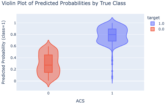
Another crucial way in which violin plots are used is to evaluate the performance of a logistic regression model by drawing the predicted probability of being the positive class or negative class, providing an easily interpretable visual of how well the model separates the two groups.

In the following example, the y-axis represents the predicted probability of having ACS (from the logistic regression model), and the color denotes the true label (e.g., a patient truly has ACS or not, based on the data). A well-performing model should have the two groups well-separated.

Figure 3.Violin plot depicting the results of a logistic regression model using high-sensitivity troponin to predict acute coronary syndrome (ACS).

Graph is authors’ own work. Note: Data is fictionalized for purposes of example and may not reflect real-world relationships.

In this violin plot (Figure 3), the negative class (no ACS) has a median predicted probability around 0.27 (red), while the positive class (ACS present) is closer to 0.8 (blue). Because these two distributions are well separated, we can conclude that the model effectively distinguishes between the two classes, indicating a good fit.⁴¹ In general, violin plots give researchers a quick check on model performance before diving into more detailed and complicated analysis. By incorporating individual raw data points, violin plots allow researchers to observe individual observations alongside the overall distribution, providing insights into data variability and potential outliers.

Sample Code (Python)

Figure 4 is a sample Python script that demonstrates how to fit a logistic regression model for ACS based on troponin, using a training and test data split, and plots the corresponding violin plot. There are numerous statistical softwares (e.g., JMP,⁴² SAS,⁴³ Stata,⁴⁴ R⁴⁵) and python packages (e.g. scikit-learn⁴⁶) that can achieve the same result, apart from the ones we have chosen here.

Figure 4.Example python script constructing a logistic regression model of ACS and troponin which prints a table of output and displays the scatterplot. Note that the dataset is a fictional example and does not reflect the real-world association between ACS and troponin. Script is author’s own work.

Conclusion

Logistic regression remains a cornerstone in clinical research for modeling binary outcomes such as disease presence or absence. Its interpretability via odds ratios and relative simplicity make it highly attractive for physicians and researchers seeking clear answers to diagnostic and prognostic questions. By understanding and addressing core assumptions (e.g., linearity in the log-odds, adequate sample size, and independence of observations), investigators can maximize both the accuracy and generalizability of their findings. Properly splitting data into training, validation, and testing sets helps guard against overfitting, while metrics such as sensitivity, precision, and the F1 score—alongside visualization tools like violin plots—allow for nuanced evaluation of model performance. When appropriately applied, validated, and interpreted, logistic regression provides a robust, clinically meaningful approach to predicting outcomes and informing evidence-based decisions.